Management Accounting Lecture
Management Accounting
1.1 Recommended Readings
Drury, C. (2012) Management and Cost Accounting, eight edition, Hampshire: Cengage Learning EMEA, Chapters 1, 2, 3 and 21.
Horngren, T. C., Datar, M. S. and Rajan, V. M. (2015) Cost Accounting: A Managerial Emphasis, fifteenth edition, London: Pearson, Chapter 5.
1.2 Learning Objectives
- Understand the meaning of management accounting.
- Understand the behaviour of the four main types of costs.
- Comprehend Absorption Costing, its benefits and limitations.
- Understand Activity Based Costing (ABC), its benefits and weaknesses.
- Comprehend Target Costing, its benefits and limitations.
1.3 What is Management Accounting?
Management accounting consists of generating accounting information in order to help management in planning, monitoring, controlling and taking decisions concerning the firm. It is important that the management accounting information given to management is relevant and is provided in a timely manner.
1.4 Cost Behaviour
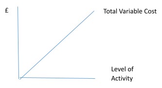
There are four main types of costs that behave in a different manner when there are changes in production. These costs are:
- Variable Cost.
- Fixed Cost.
- Stepped-Fixed Cost.
- Semi-Variable Cost.
Behaviour of Variable Cost
Behaviour of Fixed Cost
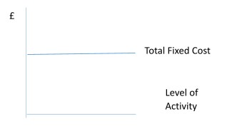
Fixed costs are not influenced by the number of units produced and are incurred even if production amounts to zero units. The fixed costs per unit decrease as the level of production increases. Examples of fixed cost comprise rent and indirect wages of supervisors.
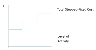
Behaviour of Stepped-Fixed Cost
Behaviour of Semi-Variable Cost
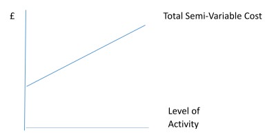
The semi-variable cost is an expenditure that includes a variable and a fixed element. Indeed, the total semi-variable cost curve does not start at zero. It starts at a higher point in order to reflect the fixed element. Electricity is an example of a semi-variable cost where there is the fixed cost element (rental of meter) and the variable cost element (consumption of electricity per unit produced).
Now, can you think of three variable costs, fixed costs, stepped-fixed costs and semi-variable costs?
1.5 Absorption Costing
This is a costing system where the full cost per unit is determined. This full cost includes direct costs and indirect costs. Direct costs are costs that can be attributed to a particular product, such as direct materials and direct labour. Indirect costs are costs that cannot be attributed to a particular product. In absorption costing it is assumed that the production overheads are influenced by one main level of activity, which can include labour hours, machine hours or number of units produced. The key steps of absorption costing are shown below:
- Costs are separated between direct and indirect costs.
- Indirect costs are allocated to one or more cost centres by using the overhead absorption rate.
- Costs present in service cost centres are apportioned to the product cost centres.
- Total costs in product costs centres are absorbed in unit costs by utilising a predetermined overhead absorption rate.
1.5.1 Example
AZ, a food manufacturer makes two types of potato chips: classic and spicy. Information pertinent to these products is shown below:
|
Items |
Classic |
Spicy |
|
Direct Material per unit |
£0.15 |
£0.20 |
|
Direct Labour per unit |
£0.06 |
£0.10 |
|
Production/Sales (units) |
300,000 |
175,000 |
|
Production Overheads |
£100,000 |
|
|
Direct Labour hours per unit |
0.03 |
0.05 |
|
Machine hours per unit |
0.09 |
0.12 |
Determine the unit cost for Classic and Spicy under absorption costing?
First one needs to determine the overhead absorption rate:

The activity level is selected by looking at the firm’s operations. AZ operations are more capital intensive because more machine hours are used per unit for both products. Thus, machine hours is selected.

The costs are now allocated to the product to determine the unit cost.
|
Costs per unit |
Classic |
Spicy |
|
Direct Materials |
£0.15 |
£0.20 |
|
Direct Labour |
£0.06 |
£0.10 |
|
Production Overheads |
£0.19 |
£0.25 |
|
Total Unit Cost |
£0.40 |
£0.55 |


1.5.2 Advantages of Absorption Costing
· Provides a more complete picture of the product cost per unit by including direct costs, and indirect variable and fixed production costs.
· Complies with the matching concept where production costs are matched with sales.
1.5.3 Disadvantages of Absorption Costing
· The absorption of fixed production costs to units is regarded as an arbitrary approach.
· One main driver is used to apportion fixed production costs between different products. This limits the accuracy of the overheads apportioned to products because overheads are influenced by more than one activity.
Now, can you think of organisations where absorption costing is appropriate?
1.6 ABC
ABC (activity based costing) is a technique, where more than one cost driver is considered in order to apportion production overheads to products. This costing method is considered a replacement to absorption costing.
The main steps of ABC are:
- The main indirect activities of the company are identified.
- Develop a cost pool for each activity.
- Identify the cost drivers for each activity.
- Determine the cost driver rate by dividing the cost pool with the cost driver.
- Use the cost driver rate in order to apportion indirect expenditure to products.
1.6.1 Example
A2Z Cars is evaluating the implementation of ABC and management decided to apportion fixed overheads in adherence to this method for the next quarter. The fixed overheads are divided into these cost pools:
Machine Costs £40,000
Component Costs £25,000
Set-Up Costs £15,000
Production Overheads £80,000
|
Cost Drivers |
Classic |
Sport |
|
Labour hours |
6,000 |
6,250 |
|
Machine hours |
18,000 |
15,000 |
|
Number of production set-ups |
2 |
3 |
|
Number of components |
5 |
8 |
Allocate the production overheads in adherence to ABC.
First one needs to identify the appropriate cost driver for each cost pool, which is done below:
|
Cost Pool |
Cost Driver |
|
Machine Costs |
Machine hours per car |
|
Component Costs |
Number of components |
|
Set-Up Costs |
Number of production set-ups |
Then one needs to determine the cost driver rate for reach cost pool:


These cost driver rates are used to apportion production overheads between Classic and Sport cars, which is done below:
|
Production Overheads |
Classic (£) |
Sport (£) |
|
Machine Costs |
(1.21 x 18,000) = 21,780 |
(1.21 x 15,000) = 18,150 |
|
Component Costs |
(1,923.08 x 5) = 9,615.40 |
(1,923.08 x 8) = 15,384.64 |
|
Set-Up Costs |
(3,000 x 2) = 6,000 |
(3,000 x 3) = 9,000 |
|
Production Overheads |
37,395.40 |
42,534.64 |
1.6.2 Advantages of ABC
- Provides more accurate cost per unit.
- Gives a better insight of the main drivers that influence indirect costs.
- ABC can be adopted on service costing as well.
1.6.3 Disadvantages of ABC
- ABC is not highly beneficial if the firm’s overheads are mainly volume related.
- There is the risk that inappropriate cost drivers are selected, which weaken the accuracy of this costing method.
- ABC is a more complicated method, which makes it more difficult to explain to stakeholders.
- It is more costly to operate an ABC system in comparison to absorption costing.
Now, can you think of organisations where ABC is appropriate?
1.7 Target Costing
This is a costing system where the target cost is derived by looking at the product selling price charged in the market and the desired profit. The main steps of target costing are:
- Identify a competitive market price.
- Derive the required profit per unit.
- Subtract the required profit from the competitive market price in order to calculate the target cost.
- Adopt cost control measures to ensure that the target cost is achieved and a competitive price is charged to customers.
1.7.1 Example
AZ is planning to launch a new product, which is the Saloon car. Competitors charge £12,000 per vehicle. Management plan to make a profit margin of 25%.
What is the target cost for the Saloon car?
First one needs to determine the target profit:
Target Profit = £12,000 x 25% = £3,000
Then one can determine the target cost, as follows:
|
Items |
£ |
|
Selling Price |
12,000 |
|
Target Profit |
3,000 |
|
Target Cost |
9,000 |
1.7.2 Advantages of Target Costing
- Stimulates cost efficiency in the organisation because efforts are made in order to achieve the target cost.
- A competitive selling price is set for the product, which is not influenced by the cost.
1.7.3 Disadvantage of Target Costing
- It is difficult to adopt target costing for organisations providing a service because it is hard to derive the competitive market price. This is due to the fact that comparison of services is more complex due to the intangibility of the service.
Now, can you think of organisations where target costing is appropriate?
2.0 MARGINAL COSTING AND BREAK-EVEN ANALYSIS
2.1 Recommended Readings
Drury, C. (2012) Management and Cost Accounting, eight edition, Hampshire: Cengage Learning EMEA, Chapters 7 and 8.
Kaplan Financial (2016) CVP Analysis (Single Product) [Online]. Available at: http://kfknowledgebank.kaplan.co.uk/KFKB/Wiki%20Pages/CVP%20Analysis%20(Single%20product).aspx.
2.2 Learning Objectives
- Calculate contribution and understand the key principles of marginal costing.
- Able to identify the variable cost per unit and fixed costs present in semi-variable costs.
- Comprehend the benefits and limitations of marginal costing.
- Calculate the break-even point and understand the break-even charts.
- Identify the implications of changes in production and costs on the break-even point.
2.3 Marginal Costing
In marginal costing fixed production costs are considered as period costs and are not included in the cost per unit rate used to value inventories of finished goods. The key equations used in marginal costing are the following:
· Sales – Variable Costs = Contribution
Contribution represents the operating profit made by the organisation before fixed costs are deducted.
· 
This ratio represents the contribution generated from sales.
· Contribution – Fixed Costs = Profit
The higher the contribution the stronger the coverage of fixed costs and the profit generated.
Marginal costing is normally used for short-term decision making like the following situations:
- Evaluate the financial feasibility of a special contract.
- Make or buy decisions.
- Determine the company’s survival point (break-even point)
- Assess the financial impact of changes in the number of units sold.
- Contribution per limiting factor.
Examples of marginal costing are given in sub-section 2.3.2 that reflect some of these situations.
In marginal costing a separation is made of variable costs and fixed costs. The high low method needs to be used in order to identify the fixed cost and the variable cost per unit present in semi-variable costs.
2.3.1 Example – High Low Method
In this method one considers the highest and lowest activity values in order to determine the variable cost per unit. The variable cost per unit is then used in order to compute the fixed costs.
|
Month |
Units Produced |
Semi-Variable Cost (£) |
|
January |
3,100 |
18,500 |
|
February |
2,990 |
17,950 |
|
March |
2,500 |
15,500 |
|
April |
3,750 |
21,750 |
|
May |
4,100 |
23,500 |
|
June |
2,804 |
17,020 |
The highest point is in May and the lowest point is in March. Therefore:
4,100 units resulted in a cost of £23,500
2,500 units resulted in a cost of £12,500
1,600 units led to additional cost of £8,000
Fixed costs will not change when production increases. Therefore, the £8,000 increase in cost due to the production of 1,600 more units is all variable cost.

One can select any point in the activity range in order to determine the fixed costs. The highest point is selected.
Total Cost £23,500
Variable Cost (5 x 4,100) £20,500
Fixed Cost £3,000
2.3.2 Examples – Marginal Costing
2.3.2.1 Make or Buy Decision
An organisation produces a type of component AR 100, which is sold at £11.95 per unit. The costs necessary to produce 100,000 units are:
|
Items |
Cost per unit (£) |
|
Direct Materials |
3.00 |
|
Direct Labour |
2.50 |
|
Variable Overheads |
1.25 |
|
Fixed Overheads |
3.20 |
|
Total Cost |
9.95 |
A supplier is offering to sell component AR 100 at a cost of £9.00 per unit. The direct labour can be used to increase the production of another component AR 110, which leads to a contribution of £3.00 per unit.
Should the company acquire the product from the supplier?
The principles of relevant costing needs to be applied in this question. In relevant costing one considers the incremental costs and revenues that will result from the decision. Opportunity cost is also considered in relevant costing, which reflects lost or additional income arising from the decision.
The costs that are not relevant to this decision are shown below:
- Direct Materials £3.00 will be avoided if the component is acquired from the supplier.
- Direct Labour £2.50 will be used for another component.
- Variable Overheads £1.25 will not be incurred if production of component AR 100 stops.
The relevant costs and revenue consist of the following:
- Fixed Overheads £3.20 will not be affected by the decision and will remain part of the total cost.
- The cost of £9.00 per unit offered by the supplier should be considered.
- The additional contribution of £3.00 should be deducted from the incremental costs.
- The component acquired from the supplier will be sold at the same selling price of £11.95.
If component AR 100 is acquired from supplier:
Revenue £11.95
Cost of component £9.00
Additional Contribution (£3.00)
Contribution £5.95
Unavoidable Fixed Costs £3.20
Profit £2.75
If component AR 100 is manufactured:
Revenue £11.95
Total Variable Costs £6.75
Contribution £5.20
Fixed Costs £3.20
Profit £2.00
If component AR 100 is acquired from the supplier it will generate additional profit of £0.75 per unit (£2.75 – £2.00). It is feasible to purchase the component from the supplier.
2.3.2.2 Change in the Number of Units Sold
In 2015 El Rasto Company that makes a single product generated the following profit:
|
|
£ |
|
Sales (units) |
70,000 |
|
Sales Revenue |
700,000 |
|
Variable Costs |
450,000 |
|
Contribution |
250,000 |
|
Fixed Costs |
236,000 |
|
Profit |
14,000 |
The company’s management is concerned about the low profit generated in 2015. The marketing director suggested to increase advertising expenditure by £15,000 and decrease the product’s selling price by 2%. This is expected to increase the number of units sold to 90,000.
Get Help With Your Accounting Coursework
If you need assistance with writing your university coursework, our professional accounting coursework writing service is here to help!
Evaluate the suggestion of the marketing director.
First one needs to determine the direct impact of this suggestion, which is on sales revenue, sales in units and fixed costs. The selling price per unit is initially determined in order to compute the sales revenue.

Decrease in Selling Price = £10 x 98% (100% - 2%) = £9.80
Sales Revenue = 90,000 x £9.80 = £882,000
Fixed Costs = £236,000 + £15,000 = £251,000
The increase in sales will lead to higher production, which increases the variable costs. Therefore, one needs to compute the variable costs per unit in order to determine the new variable costs.

Variable Costs = 90,000 x £6.43 = £578,700
Now one can prepare the profit statement under marginal costing, which is shown below:
|
|
£ |
|
Sales Revenue |
882,000 |
|
Variable Costs |
578,700 |
|
Contribution |
303,300 |
|
Fixed Costs |
251,000 |
|
Profit |
52,300 |
The suggestion of the marketing director will increase El Rasto’s profitability by £38,300 (£52,300 - £14,000). Thus, the suggestion is financially feasible.
2.3.3 Advantages of Marginal Costing
- Profits are not distorted by changes in inventory levels because fixed costs are considered as period costs.
- Technique that helps to generate valuable information for decision making, such as contribution, break-even point and margin of safety.
2.3.4 Disadvantages of Marginal Costing
- In practice sometimes it is difficult to identify the fixed and variable elements present in costs.
- Unrealistic assumptions are taken in marginal costing, such as that the variable cost per unit will always remain the same. Variable costs may decrease over time due to improved efficiency resulting from better skills by employees.
- Fails to consider qualitative factors like product quality and company’s reputation, which are also important for the company.
Now, can you identify the main differences between absorption costing and marginal costing?
2.4 Break-Even Point
The break-even point is the point where the revenue generated by the company is equal to the costs incurred. In marginal costing this is the point where the contribution is equal to the fixed costs. The break-even point is calculated via the following equations:


2.4.1 Example
A company is planning to market a new product at a selling price of £25 per unit. The fixed costs amount to £70,000 and the contribution per unit is £14. Determine the break-even point in units and £.


2.4.2 Break-Even Charts
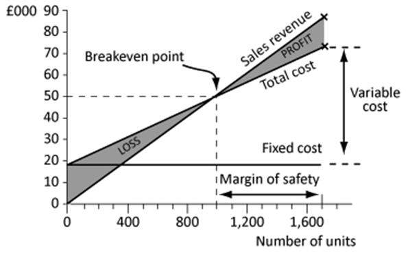
Traditional Break-Even Chart
Source: Kaplan Financial, 2016.
The break-even point is the point where the sales revenue meets the total cost. At this point the profit generated amounts to zero. The total cost includes the fixed cost and the variable cost. However, the fixed cost is also shown in the graph, as a horizontal line. The traditional break-even chart also shows the margin of safety, which is the difference between the sales revenue and the break-even sales. A product with a low margin of safety holds a high business risk because losses can be incurred easily if sales decrease.
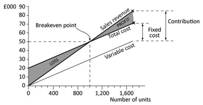
The traditional break-even chart fails to show the contribution. This problem is mitigated by preparing the contribution break-even chart, which is shown below:
Source: Kaplan Financial, 2016.
The introduction of the variable cost helps to determine the contribution, which is the difference between sales revenue and variable cost. The fixed cost is the gap between the total cost and variable cost.
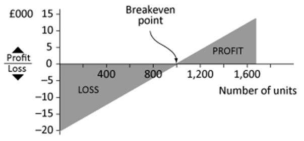
Profit-Volume Chart
Source: Kaplan Financial, 2016.
The profit-volume chart indicates the sales volumes that will lead to a loss and the volumes, which will result in profit.
2.4.3 Uses of Break-Even Analysis
- The main use of break-even analysis is that management can observe the impact of changes in sales volume and costs on productivity.
- The break-even point is also useful to determine the margin of safety and evaluate the risk of the product.
2.4.4 Limitations of Break-Even Analysis
- In practice, sales are not always proportional to the increase in the number of units sold.
- There may be stepped-fixed costs, which are not reflected in the traditional break-even chart.
- In practice variables costs, total costs and total income are not a straight line.
- It is assumed that changes in the number of units produced and sold are the only factors that affect revenues and costs. In practice this is not always the case. For example, employee motivation may lead to changes in variable costs.
- Break-even analysis is more appropriate for the short-term.
3.0 CAPITAL BUDGETING
3.1 Recommended Readings
Atrill, P. and McLaney, E. (2015) Accounting and Finance for Non-Specialists, ninth edition, London: Pearson, Chapter 10.
Horngren, T. C., Datar, M. S. and Rajan, V. M. (2015) Cost Accounting: A Managerial Emphasis, fifteenth edition, London: Pearson, Chapter 21.
3.2 Learning Objectives
- Calculate project’s cash flows.
- Calculate and describe the following methods:
- Accounting Rate of Return (ARR)
- Payback Period (PP)
- Discounted Payback
- Net Present Value (NPV)
- Profitability Index (PI)
- Internal Rate of Return (IRR)
- Evaluate the feasibility of capital projects.
- Adopt sensitivity analysis.
- Understand the cost/benefit analysis.
3.3 Project Evaluation
Capital projects require substantial investments of money and have a long-term influence on the organisation. Therefore, it is imperative that management selects the right projects for the company.
3.4 Capital Budgeting Methods
There are a number of capital budgeting methods used in order to evaluate financial feasibility of capital projects.
3.4.1 ARR
The ARR represents the average operating profit the organisation will generate from the project. This is calculated as follows:

3.4.1.1 Example:
An organisation will acquire a new machine costing £150,000 with a residual value of £10,000. This new machine will increase operating profit by the following figures for the next five years: £30,000, £25,000, £15,000, £32,000 and £26,000. Management expect a minimum ARR of 25%.
Evaluate this project by using the ARR.


The following factors should be considered in order to evaluate the project:
- To be accepted the project needs to achieve the target ARR of the organisation. Therefore, this project is feasible because the ARR of 32% is higher than the minimum ARR of 25%.
- For mutually exclusive projects the project with the highest ARR is selected.
Mutually exclusive projects arise when the organisation cannot undertake all the projects and needs to select the best one.
3.4.1.2 Advantages of ARR
- Simple method to understand and calculate.
- Based on accounting profit, which is available in the financial statements
3.4.1.3 Disadvantages of ARR
- Profit is an arbitrary and subjective figure.
- Ignores the time value of money principle.
3.4.2 PP
This method determines the time taken for the cash flows to cover the initial capital cost of the project. The lower the PP the better the capital project.
3.4.2.1 Example
A company is evaluating a new project that involves the following cost and operating profits:
|
Year |
Items |
£’000 |
|
0 |
Cost of Machine |
(150) |
|
1 |
Operating Profit |
50 |
|
2 |
Operating Profit |
45 |
|
3 |
Operating Profit |
52 |
|
4 |
Operating Profit |
50 |
|
5 |
Operating Profit |
49 |
The machine has a useful life of five years and no residual value. The operating profit includes the depreciation charge.
Evaluate this project by using the PP.
PP is based on cash flows and thus one needs to add back the depreciation, which is a non-cash expense.

|
Year |
Cash Inflow/Outflow |
£’000 |
|
0 |
Cost of Machine |
(150) |
|
1 |
Cash Inflow (50 + 37.5) |
87.5 |
|
2 |
Cash Inflow (45 + 37.5) |
82.5 |
|
3 |
Cash Inflow (52 + 37.5) |
89.5 |
|
4 |
Cash Inflow (50 + 37.5) |
87.5 |
|
5 |
Cash Inflow (49 + 37.5) |
86.5 |
The cumulative cash flows need to be calculated in order to find the year where the cost of machine is covered.
|
Year |
Cash Flow £ |
Cumulative Cash Flow £ |
|
0 |
(150) |
-150 |
|
1 |
87.5 |
(87.5 – 150) = -62.5 |
|
2 |
82.5 |
(82.5 – 62.5) = 20 |
The cost of machine is covered in year 2. However, in year 2 an annual positive cash flow of £20,000 is expected. Therefore, one needs to determine the number of days necessary to cover the negative £62,500 at the beginning of year 2.

The following factors should be considered in order to evaluate the project:
- The PP should be lower than the life of the project. Therefore, the project considered in this example is financially feasible.
- For mutually exclusive projects the project with the lowest PP is selected.
3.4.2.2 Advantages of PP
- Easy to calculate and understand.
- Considers cash flow to evaluate the project and avoids subjective figures included in accounting profit.
- Decreases risk by favouring projects that give a quick return.
- Favours projects that give fast cash flow. This improves the firm’s liquidity.
3.4.2.3 Disadvantages of PP
- Ignores the time value of money principle.
- Does not consider the total financial impact of the project.
3.4.3 Discounted Payback
This is similar to the PP except that future cash flows are discounted. Such discounting is in line with the time value of money principle, which means that £1,000 received today have more value than £1,000 received next year. Discounted cash flows represent today’s value of future cash flows. Such principle is important because it helps to evaluate all competing projects on the same basis.
3.4.3.1 Example
The same example considered in 3.4.6 is used and the cost of capital is at 10%.

|
Year |
Cash Flow |
10% Discount Factor |
Discounted Cash Flow |
Cumulative Cash Flow |
|
0 |
(150) |
1.0000 |
-150 |
-150 |
|
1 |
87.5 |
0.9091 |
79.6 |
(79.6 – 150) = -70.4 |
|
2 |
82.5 |
0.8264 |
68.2 |
(68.2 – 70.4) = -2.2 |
|
3 |
89.5 |
0.7513 |
67.2 |
(67.2 – 2.2) = 65 |

The project is evaluated under the same criteria used for the PP. Thus, under the discounted payback the project considered above is still financially feasible because the capital cost will be covered during the project’s life.
3.4.3.2 Advantages of Discounted Payback
- Complies with the time value of money principle.
- Uses cash flow in order to evaluate the project.
- Decreases risk by favouring projects that give a quick return.
- Favours projects that give fast cash flow, which can improve the firm’s liquidity.
3.4.3.3 Disadvantage of Discounted Payback
- Does not consider the total financial impact of the project.
3.4.4 NPV
NPV represents the financial wealth that the company will make from the project. The NPV figure is derived by considering all the relevant cash inflows and outflows, which are discounted by the cost of capital.
3.4.4.1 Example
The following cash flows are anticipated for a project:
|
Year |
0 |
1 |
2 |
3 |
4 |
|
Cash Inflow/(Outflow) |
(£400) |
£100 |
£150 |
£300 |
£400 |
The cost of capital is at 10%.
Evaluate this project by utilising the NPV.
|
Year |
Cash Inflow/(Outflow) |
Discount Factor at 10% |
Present Value |
|
0 |
(£400) |
1.0000 |
(£400) |
|
1 |
£100 |
0.9091 |
£90.91 |
|
2 |
£150 |
0.8264 |
£123.96 |
|
3 |
£300 |
0.7513 |
£225.39 |
|
4 |
£400 |
0.6830 |
£273.20 |
|
NPV |
£313.36 |
||
The following factors should be considered in order to evaluate the project:
- Projects with a positive NPV are financially feasible. Therefore, the project considered in this example is feasible.
- For mutually exclusive projects the project with the highest NPV is chosen.
3.4.4.2 Advantages of NPV
- Complies with the time value of money principle.
- Considers all the financial wealth emerging from the project.
- Uses cash flow and avoids the subjectivity present in accounting profit.
3.4.4.3 Disadvantages of NPV
- Complex to calculate especially to determine the cost of capital.
- Method is more complicated and difficult to understand.
3.4.5 IRR
IRR represents the discount rate that will lead to a zero NPV. Changes in the cost of capital will lead to different NPVs. IRR calculates the maximum cost of capital that a particular project can bear. The IRR is normally found by trial and error.
3.4.5.1 Example
The same example considered in 3.4.13 is used.
|
Year |
Cash Inflow/(Outflow) |
Discount Factor at 34% |
Present Value |
|
0 |
(£400) |
1.0000 |
(£400) |
|
1 |
£100 |
0.7463 |
£74.63 |
|
2 |
£150 |
0.5569 |
£83.54 |
|
3 |
£300 |
0.4156 |
£124.68 |
|
4 |
£400 |
0.3102 |
£124.08 |
|
NPV |
£6.93 |
||
For IRR one needs to identify two discount rates. One that provides a low NPV that is close to zero and the other discount rate that leads to a negative NPV. At 34% the NPV is very small and close to zero. A negative NPV will result at a discount rate of 35%. This is computed below in order to identify the point where NPV amounts to zero:
|
Year |
Cash Inflow/(Outflow) |
Discount Factor at 35% |
Present Value |
|
0 |
(£400) |
1.0000 |
(£400) |
|
1 |
£100 |
0.7407 |
£74.07 |
|
2 |
£150 |
0.5487 |
£82.31 |
|
3 |
£300 |
0.4064 |
£121.92 |
|
4 |
£400 |
0.3011 |
£120.44 |
|
NPV |
(£1.26) |
||

The following factors should be considered in order to evaluate the project:
- The project should be implemented if the IRR is higher than the cost of capital. In example 3.4.13 the cost of capital was 10%. Therefore, the project is financially viable.
3.4.5.2 Advantages of IRR
- Determines the return derived from the initial investment.
- Follows the time value of money principle.
3.4.5.3 Disadvantages of IRR
- IRR provides a relative measures of the project’s feasibility.
- This method is unable to provide an IRR or can result in multiple IRRs when the project has non-conventional cash flows. Non-conventional cash flows mean that cash outflows does not arise only when the project is implemented (year 0).
- Not appropriate to evaluate mutually exclusive projects because it can select a project that leads to lower total financial wealth.
Get Help With Your Accounting Coursework
If you need assistance with writing your university coursework, our professional accounting coursework writing service is here to help!
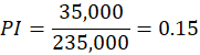
3.4.6 PI
PI indicates the proportion of pay off return derived from the initial investment. This is computed via the following equation:

3.4.6.1 Example
A project is envisaged to lead a NPV of £35,000. The capital cost amounts to £235,000.
Assess this project by using the PI.
The following factors should be considered in order to evaluate the project:
- The PI should be higher than 1 in order to accept the project. Therefore, the project in this example is not financially feasible.
3.4.6.2 Advantages of PI
- Utilises NPV, which is a calculation based on cash flows.
- Follows the time value of money principle.
3.4.6.3 Disadvantages of PI
- PI provides a relative measure and is unable to show the overall impact on the firm’s financial wealth.
- This method is not appropriate to rank mutually exclusive projects because it gives a relative measure.
Now, can you identify the best capital budgeting method that can be used by organisations engaged in manufacturing?
3.4.7 Sensitivity Analysis
Sensitivity analysis is used to deal with the uncertainty of projects, which ultimately result in the risk that the company is unable to achieve the desired return. Sensitivity analysis comprises changing key values of the project like sales volume, selling price, cost of capital and incremental cost and see the impact of the change on the NPV.
3.4.7.1 Example
A company intends to buy a machine costing £150,000, which is expected to lead to the following cash inflows: Year 1 £50,000; Year 2 £52,000; Year 3 £79,000 and Year 4 £90,000. A NPV of £59,254.83 is envisaged at 10% cost of capital.
What is the impact of a 20% increase in the cost of capital?
|
Year |
Cash Inflow/(Outflow) |
Discount Factor at 12% |
Present Value |
|
0 |
(£150,000) |
1.0000 |
(£150,000) |
|
1 |
£50,000 |
0.8929 |
£44,645.00 |
|
2 |
£52,000 |
0.7972 |
£41,454.40 |
|
3 |
£79,000 |
0.7118 |
£56,232.20 |
|
4 |
£90,000 |
0.6355 |
£57,195.00 |
|
NPV |
£49,526.60 |
||
NPV will decrease by £9,728.23 if the cost of capital increased by 20% but the project will still remain financially sound.
3.4.8 Cost/Benefit Analysis
This analysis is normally applied to capital projects where attention is devoted to the costs stemming from the project and the benefits anticipated from the project. If the benefits are greater than the costs the project is feasible and should be undertaken. The benefits and costs considered should not only be financial. Qualitative factors should also be considered. This leads to a problem because qualitative factors are more difficult to assess in an objective manner.
Sunk costs should be excluded from the cost/benefit analysis. Sunk costs are irrelevant costs because these costs have already been incurred and the acceptance or rejection of the project will have no impact on these costs. For example, an organisation has made a market research costing £40,000 in order to identify the demand for a new product. This is a sunk cost because such cost cannot be influenced by the decision taken by management.
3.5 BUDGETING AND STANDARD COSTING
3.5.1 Recommended Readings
Atrill, P. and McLaney, E. (2015) Accounting and Finance for Non-Specialists, ninth edition, London: Pearson, Chapter 9.
Horngren, T. C., Datar, M. S. and Rajan, V. M. (2015) Cost Accounting: A Managerial Emphasis, fifteenth edition, London: Pearson, Chapter 6.
3.5.2 Learning Objectives
- Understand budgetary planning and control.
- Identify the strengths and limitations of budgeting.
- Describe the different types of budgeting systems.
- Understand the meaning of standard costing.
- Explain the different types of standards.
- Understand the implications of variance analysis as a control tool.
3.5.3 Budgetary Planning and Control
Budgets serve two purposes, which are to help management in planning and control. Budgets are short-term plans that reflect the corporate objectives of the organisation. A system of responsibility accounting is adopted by organisations using budgeting where each department is responsible for a specific budget. The performance of the departmental manager will be evaluated by looking at his/her ability to meet the budget set. Budgetary control involves a philosophy known as management by exception. This means that the attention of senior management is directed to exceptions, which consist of deviations from the budgets set. Therefore, there is a system where the actual costs are compared with the budgeted costs and significant variances are investigated in order to identify weaknesses or strengths.
3.5.4 Benefits of Budgets
- Provide a system where the strategic objectives of the organisation are translated in clear measurable targets.
- Budgets promote coordination between the different departments of the organisation.
- The adoption of management by exception helps managers to focus on the most important aspects of the organisation.
- Budgets enhance control in the firm because all functions are monitored in a systematic manner. This leads to the identification of weaknesses, which are removed in order to improve efficiency, productivity and effectiveness.
- An appropriate budgeting system can improve the cash management and working capital of the organisation.
- The involvement of managers and employees in a budgeting system can result in motivation, which enhances the firm’s operations. This is especially the case when a bonus system is amalgamated with the budgeting system.
3.5.5 Limitations of Budgets
- The preparation of budgets is time consuming for managers especially if a participatory system of budgeting is adopted. In a participatory system the operational managers prepare the functional budgets with senior management.
- Promotes inflexibility in the organisation where emphasis is placed on short-term financial targets.
- Budgetary slack can occur when a participatory system of budgeting is used. In budgetary slack the operational manager tries to underestimate expected revenue or overestimate anticipated costs in order to make easier targets.
- Focus is made on financial targets and there is the risk that qualitative features like the reputation of the organisation are neglected.
- There is the risk that the organisational structure is inappropriate for the budgeting system set. For example, a participatory style of budgeting is used in an organisation that holds a bureaucratic organisational structure. This will prevent the organisation to achieve the benefits of budgeting because the organisational structure does not comply with the budgeting system selected.
- Budgeting may lead to demotivation when the working relationships between managers and employees are poor.
- Budgeting may be erroneously considered a substitute for good management practice.
3.5.6 Budgeting Systems
There are six main budgeting systems, which are explored in this subsection. These budgeting systems have different benefits and limitations, and management should select the most appropriate one for the organisation.
3.5.6.1 Top Down Budgeting
This is a budgeting system where the budgets are prepared by senior management and they are imposed on the operational managers and employees.
3.5.6.1.1 Advantages
- Budgets can be more strategically focused because these are prepared by senior managers who are the individuals that prepare the strategic plan.
- Top down budgeting is less time consuming than other budgeting systems.
- Provides more realistic budgets when operational managers are new and they have limited knowledge for budget preparation.
3.5.6.1.2 Disadvantages
- Can stimulate inertia and demotivation among operational managers and employees especially when tight budgets are set.
- Budgets prepared may neglect important operational aspects.
3.5.6.2 Bottom Up Budgeting
In this budgeting system the operational managers are able to participate in the preparation of the budget. This budgeting system is also known as participative budgeting.
3.5.6.2.1 Advantages
- Helps operational managers to understand better the targets behind the budgets set.
- Enhances communication between departments.
- Senior management can focus on the development of corporate strategies.
- Increases motivation because operational managers have a feeling of ownership because they were engaged in the budget preparation.
3.5.6.2.2 Disadvantages
- This budgeting system decreases the control senior managers have on the firm’s operations.
- Inexperienced operational managers may propose unrealistic budgets.
- The preparation of the budgets is more time consuming.
- There is the risk of budgetary slack.
- There is the risk of dysfunctional behaviour, which arises when the budgets are not in adherence to the corporate objectives of the organisation.
3.5.6.3 Incremental Budgeting
This budget is prepared by adding an incremental amount to the budget of the previous period or the actual results. For example, in the previous period’s budget it was estimated that material costs would amount to £27,000. An additional 10% is added in the current budget leading to material costs of £29,700.
3.5.6.3.1 Advantages
- Simple and fast budgeting system.
- Appropriate for organisations that operate in a stable business environment.
3.5.6.3.2 Disadvantages
- Operational managers will be stimulated to spend all the budget in order to ensure that a percentage increase is provided in the next budget.
- It is based on previous budgets that may hold inefficiencies and uneconomic activities. For example, the organisation may continue acquiring a component from a supplier despite it is more economically feasible to manufacture it.
3.5.6.4 Zero-Based Budgeting (ZBB)
ZBB is the opposite of incremental budgeting where each cost has to be justified by the manager before it is included in the budget. Indeed, ZBB starts at a cost of zero.
3.5.6.4.1 Advantages
- Helps in the identification of inefficiencies.
- Stimulates managers to be more informative about the costs that are adding value to the organisation and are justifiable.
- Promotes cost control in the organisation.
- Improves understanding of cost behaviour in the firm’s operations.
3.5.6.4.2 Disadvantages
- Preparation of ZBB is time consuming.
- Places considerable focus on short-term targets, thereby giving lower importance to long-term objectives.
- ZBB may be considered a very rigid budgeting system that leads to demotivation.
- Difficult to evaluate costs especially when qualitative benefits need to be taken into account.
3.5.6.5 Rolling Budgets
A rolling budget is continuously kept updated by preparing an additional budgeting report. For example, if the budgets are prepared on a quarterly basis an additional quarter is done.
3.5.6.5.1 Advantages
- More accurate budgets that enhance planning and control.
- Stimulates managers to evaluate the budget estimates when preparing the rolling budget.
- Helps to decrease budgetary slack.
3.5.6.5.2 Disadvantages
- More time consuming and costly for the organisation.
- Employees may become demotivated if the budget targets are consistently altering.
- May deviate the attention of management from control to budget preparation. Control is an essential feature of budgeting.
3.5.6.6 Activity-Based Budgeting
This budgeting system is based on the principles of ABC where budgeted expenditure is derived by looking at the activities the firm undertakes to develop the product.
3.5.6.6.1 Advantages
- Places emphasis on overhead activities, which can be a significant part of the firm’s total operating expenditure.
- Helps in the identification of the cost drivers, which are the main factors that influence the cost.
3.5.6.6.2 Disadvantages
- Requires considerable time for the identification of the main activities and cost drivers.
- Overhead expenditure is often non-controllable in the short-term. Therefore, there is little control that can be adopted for such expenditure, which limits the usefulness of budgets.
3.5.7 Standard Costing
Standard costing entails setting predetermined estimates for product and service costs, recording actual costs and compare the actual figures with these estimates. The resulting figure is the variance, which is a useful tool to outline problems in efficiency and productivity. There are four types of standards:
- Ideal Standard – this standard is based on the assumption that there is no idle time, wastage and other form of inefficiency. Thus, it is very difficult for employees to achieve the ideal standard and such a standard can be considered a long-term target for the organisation.
- Attainable Standard – in this standard allowance is made for idle time, wastage and breakdowns. However, a good level of efficiency needs to be achieved in order to achieve this standard.
- Current Standard – this standard reflects the current efficiency and productivity of the organisation. Such a standard is appropriate when conditions are stable and there is no need for additional efficiency and productivity.
- Basic Standard – this is a long-term standard that is utilised in order to indicate trends in costs like wage rate and price of materials. The basic standard is also utilised in order to develop the current standard.
What is the support that standard costing provides for budget preparation?
3.5.7.1 Ideal, Attainable or Current Standard?
An ideal standard may result in frustrated managers and demotivated employees because it is very difficult to attain. A current standard is also unable to motivate staff because such a level of efficiency and productivity has already been reached. An attainable standard is more appropriate because it is not very difficult to achieve but additional effort is still needed by staff in order to be attained.
3.5.8 Variance Analysis
The scope of variances is to provide financial figures which indicate that the actual performance in that area was different from the budget. Variances are prepared for sales, direct materials, direct labour, variable overheads and fixed overheads. Two types of variances are investigated for each category:
- Price variance, which shows the difference between the actual price to the standard cost.
- Efficiency variance, which reflects the difference between the actual quantity to the standard quantity for actual production.
Variances need to be investigated in order to identify the reason causing that variance and adopt control measures where appropriate. Such investigations lead to the identification of controllable and uncontrollable variances. Controllable variances are within the manager’s control and action should be taken to mitigate such variances. Uncontrollable variances cannot be altered by management and the standard costs should be adjusted to reflect such variances.
Cite This Module
To export a reference to this article please select a referencing style below: