Implementation of Wireless Receiver Algorithms
| ✅ Paper Type: Free Essay | ✅ Subject: Technology |
| ✅ Wordcount: 2859 words | ✅ Published: 14 Aug 2017 |
Figure 1 System Specifications (Tsimenidis, 2016)
Figure 2 Message format (Tsimenidis, 2016)
Figure 3 Non-coherent receiver (Tsimenidis, 2016)
Figure 4 Coherent receiver (Tsimenidis, 2016)
Figure 5 Receiver Front-End (Tsimenidis, 2016)
Figure 6 Frequency response of a passband filter (Tsimenidis, 2016)
Figure 7 Band-pass filter response
Figure 8 Band-pass filter input/output
Figure 9 Implemented DPSK demodulator (Tsimenidis, 2016)
Figure 10 Low-pass filter input/output
Figure 11 Optima sample time diagram
Figure 12 Symbol with 40 samples (Tsimenidis, 2016)
Figure 13 Early-Late sample at an arbitrary point (Tsimenidis, 2016)
Figure 14 Early-Late sample at the maximum point of power (Tsimenidis, 2016)
Figure 15 Early-Late symbol synchronization input/output
Figure 16 Result of non-coherent receiver detection
Figure 17 IQ Downconverter (Tsimenidis, 2016)
Figure 18 Sine and cosine table graphs
Figure 19 Index control flow (Tsimenidis, 2016)
Figure 20 Filter comparison (Tsimenidis, 2016)
Figure 21 Down-conversion: x3I vs. x3Q counter clockwise
Figure 22 Down-conversion: x4I vs. x4Q counter clockwise
Figure 24 Averaging approach to overcome the jitter (Tsimenidis, 2016)
Figure 25 Code to solve the jitter
Figure 26 Principle of the differential detector (Tsimenidis, 2016)
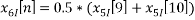
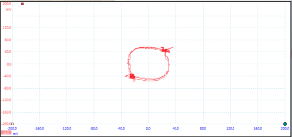
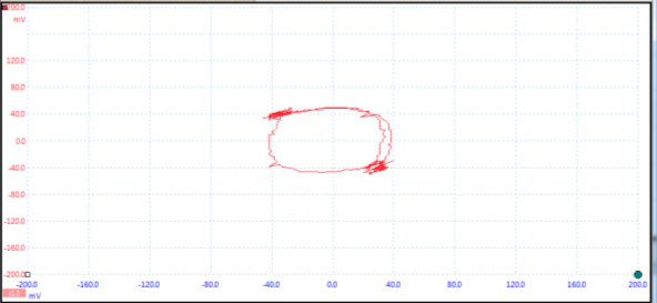
Figure 27 Constellation without Phase Offset (dI Vs dQ)
Figure 28 Result of coherent receiver detection using differential coherent demodulator
Figure 29 BPSK and DPSK BER comparison (Tsimenidis, 2016)
Figure 30 Costas Loop algorithm (Tsimenidis, 2016)
Figure 31 Costas loop: yQ vs. yI
Figure 32 Message obtained using Costas loop
Figure 33 BER comparison of different modulation schemes and techniques (Sklar, 1983)
This project is focused on implementing and coupling several functional blocks that will allow us to detect, extract and decode a wireless message that is being broadcasted in the Merz lab of computers. In the following sections, we will find the implementations of coherent and non-coherent receivers.
In the section 1 we define the basic background knowledge that will be commonly used in the posterior phases of the report. We define the basic structure and features of the transmitter as well as the message format that the system is intended to detect. Finally, we define what is a coherent and a non-coherent system and provide a classification about the different techniques.
In the section 2 we will analyse the non-coherent receiver implementation from the message acquisition, going to the filter section, signal scaling and refinement, using a DPSK demodulator to define the probable symbols represented, then establishing a synchronization for the symbol and finally presenting the message obtained.
The section 3 will focus in the realization of a coherent receiver, considering two possible variations on this type of implementation: the first will be developed using a differential coherent demodulator, in this technique we will not recover the carrier signal. The second implementation of this receiver, will be done using a carrier recovery technique, which is in this case a Costas Loop Algorithm.
Some common blocks are done in all the possible implementations that were carried out during this project: the first is the receiver front-end which is the responsible to acquire and prepare the signal for the posterior processing. To recover the symbol synchronization, we use a technique called early-late gate, this will let us know what is the most convenient instant of the time to sample the signal. For the case of coherent signal, we must adapt this technique to apply it separately for the signal I (in-phase) and Q (quadrature).
The section 4 contains analysis, conclusions and discussions of the results obtained during the realization of the phases.
The last sections of the report detail the references used for further explanations and the different programs used for implementing each block.
In each section, we include little further explanations that could be referred to understand the steps and details that have been done in the corresponding section.
1. Background knowledge
1.1. Aims and objectives
The focus of this project is to demonstrate the implementation and the behaviour of data links using Radio Frequency as media and different techniques. Basically, we use two techniques: coherent and non-coherent implementations. A further explanation of these techniques will be done in the following sections.

A second implementation of a coherent receiver will be carried out by using a phase recovery technique with the Costas Loop and coupling the posterior phase to this block.
The specifications of the system to be implemented could be defined as a set of blocks connected as follows:
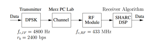
Figure 1 System Specifications (Tsimenidis, 2016)
Where the transmitter has been already implemented, therefore the work will be carried out in the receiver algorithm to obtain the final data, which of course must be in a human readable format.
We also must consider that the format of the message that is being broadcasted wirelessly in the Merz lab has the following format:
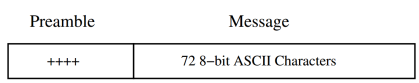
Figure 2 Message format (Tsimenidis, 2016)
1.2. Digital modulation
The digital modulation process refers to a technique in which the digital representation of the information is embedded in a signal, a carrier typically a sinusoidal signal, in such a way that this information will modify an established parameter of the signal.
We can define a sinusoidal carrier in a general way as a signal that will correspond to the equation:

Where the information could be embedded in  this will be called amplitude modulation, if the parameter
  this will be called frequency modulation and finally the phase modulation will be obtained if we embed the data in the expression
 .
.
Regard to the symbol  this is called the angular frequency, it is measured in radians per second, this is related to the frequency (f) expressed in Hertz by the expression
 .
.
1.3. Coherent and non-coherent detection
Considering the receiver side, we can classify the demodulation or detection based on the use of the carrier’s phase information in the process of information recovery. In the case that the receiver uses this information to detect the signals it will be called coherent detection, and non-coherent detection otherwise. This are also called synchronous and asynchronous detection, respectively.
|
Coherent |
Non-Coherent |
|
Phase Shift Keying (PSK) |
Diferential Phase Shift Keying (DPSK) |
|
Frecuency Shift Keying (FSK) |
Frecuency Shift Keying (FSK) |
|
Amplitude Shift Keying (ASK) |
Amplitude Shift Keying (ASK) |
|
Continuous Phase Modulation (CPM) |
Continuous Phase Modulation (CPM) |
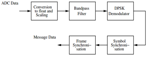
Figure 3 Non-coherent receiver (Tsimenidis, 2016)
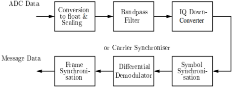
Figure 4 Coherent receiver (Tsimenidis, 2016)
2. Non-coherent receiver
2.1. Receiver Front-End
This segment of the non-coherent receiver will consist of the first two blocks, which are common for both coherent and non-coherent implementations.
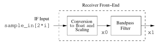
Figure 5 Receiver Front-End (Tsimenidis, 2016)
The first block is the responsible to take a sampled input expressed as bits, represent it as a float number and then normalise it to a range +/- 1.0.
The second stage applies a bandpass filter to the signal, this will attenuate the parasites components of frequency that could contaminate the signal that we received.
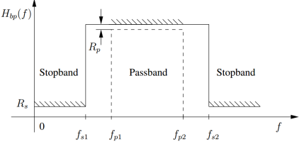
Figure 6 Frequency response of a passband filter (Tsimenidis, 2016)
To design the passband filter we must consider the following information: let  = 4800 Hz, data rate
  = 2400 bps and sampling frequency
  = 48000 Hz.
These assumptions, led us to the following results:
Lower passband cut-off frequency:
 = –
= –  = 3600 Hz
Upper passband cut-off frequency:
 = + = 6000 Hz
Lower stopband cut-off frequency:
 = –
= –  = 1200 Hz
Upper stopband cut-off frequency:
 = + = 8400 Hz
The implementation of the filter will be done using the sptool command of Matlab, using the above defined values as parameters for the filter.
The following figure shows the result obtained in the realization of the lab, considering the number of filter coefficients of 101.
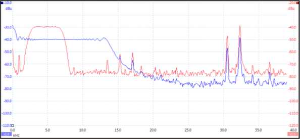
Figure 7 Band-pass filter response
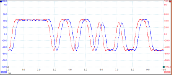
Figure 8 Band-pass filter input/output
2.2. DPSK demodulator
To implement the non-coherent detection, we are going to use a DPSK demodulator, which was previously categorized as a non-coherent technique.
The DPSK demodulator will take advantage of two basic operation that occur on the transmitter: the first is the differential encoding, and the second is the phase-shift keying. In the transmitter, the signal will be advanced in phase, with respect to the current signal, if the symbol to be sent is 0, and the phase will be preserved if the bit corresponds to 1. In the side of the receiver, we have memory that will be able to compare the phase of two successive bit intervals, i.e. it determines the relative difference in phase of these two, determining the correspondent symbols without the need of having information about the phase of the signal in the transmitter.
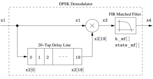
Figure 9 Implemented DPSK demodulator (Tsimenidis, 2016)
The FIR matched filter block will correspond to a low-pass filter, this is required because the demodulation process, as it is a multiplication between two sinusoidal signals, will generate a low-band signal and a high-band signal, where the second one should be filtered.
2.3. Symbol synchronisation
The symbol synchronisation, also called symbol timing, is a critical process that consists in the continuous estimation and update of information of the symbol related to its data transition epochs. This is a critical process that must be conducted to keep the communication accuracy in acceptable levels.
Broadly speaking, the synchronization techniques could be classified in two groups: open-loop and closed-loop. The chosen technique for this project corresponds to the Early-Late Symbol Synchronization which is a closed-loop type. The most popular technique is the closed-loop synchronization because “Open-loop synchronizer has an unavoidable nonzero average tracking error (though small for large SNR, it cannot be made zero), a closed-loop symbol synchronizer circumvents this problem.”(Nguyen & Shwedyk, 2009)
The corresponding results of the output of the demodulator are the following figures, these corresponds to the signals before and after the signal is filtered with the FIR low-pass filter.
Notes:
- The curve in blue corresponds to the signal containing the high-frequency parasite component, and the curve in red shows the result of filtering the high frequency component, i.e. this is the output signal of the filter.
- The symbol correspondence is: symbol 0 for positive numbers, and symbol 1 for negative magnitudes.
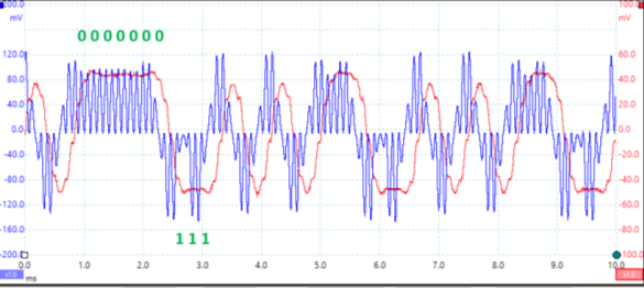
Figure 10 Low-pass filter input/output
2.3.1. Early-late Symbol Synchronization (Reed, 2002)
The algorithm Early-late used for synchronization is supported by the idea that the sample of a symbol must be taken in the time where the energy is maximum, this will warranty a minimum error probability.
This algorithm exploits the symmetry of the signal, neglecting the distortion and noise. Considering the following figure, we can see that the optimal time to take the sample, identified as T, should be in the halfway between two points T0 + d and T0 – d, if the power in the T0 + d and T0 – d is, ideally, the same.
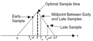
Figure 11 Optima sample time diagram
Suppose the following figure shows a symbol, we can notice that if we take an arbitrary sample, e.g. n=3 and depending on the thresholds, could be wrongly interpreted as 0, however the most appropriated value is 1.
Figure 12 Symbol with 40 samples (Tsimenidis, 2016)
With a buffer size of 20 registers, we can notice that in the following figure the power levels of the signal for n=0 and n=19 are different, then we need to move the whole buffer one space to the right.
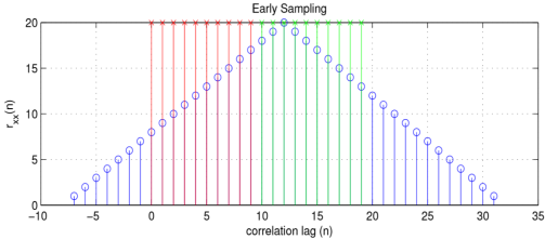
Figure 13 Early-Late sample at an arbitrary point (Tsimenidis, 2016)
If we continue with the iteration and we follow the rules described in the flow diagram, we will converge in a finite number of iterations, where we can see that the result is located as expected, this could be seen in the following figure.
Figure 14 Early-Late sample at the maximum point of power (Tsimenidis, 2016)
The results of the application of this algorithm for our case are shown in the following figure:
Note:
- The signal in red is the input of the early-late symbol synchronization block and the signal in blue is the value of Em that will finally determine the value that the symbol is representing, in each case.
Figure 15 Early-Late symbol synchronization input/output
2.4. Frame synchronisation
As was stated in the in the background section, the message frame will begin with the characters “++++” and the message has 72 bytes encoding the message using a ASCII characters. Therefore, this section will deal with two tasks: (1) Detect the message preamble and (2) Decode byte per byte of the data contained in the payload.
After the preamble section, we will detect 576 bits, corresponding to the 72 bytes that correspond to the ASCII characters. These characters will be dumped into an executable file that will then show the message that has been detected and decoded.
The specific implementation of the algorithm is attached in the appendix section of this report.
2.5. Results and evaluation
The result of applying the steps described in the sections from 2.1 to 2.4, we obtain the message, getting the result showed in the next figure:
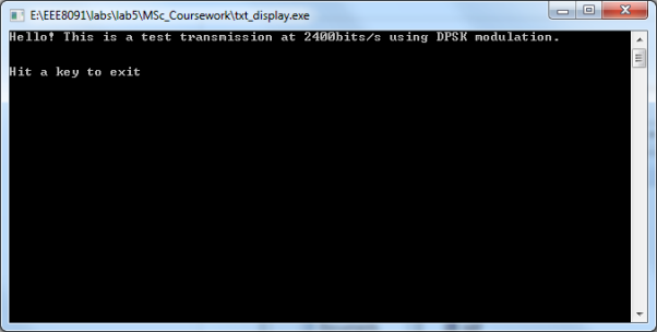
Figure 16 Result of non-coherent receiver detection
3. Coherent receiver
The coherent receiver, also called synchronous receiver, implies certain degree of agreement or knowledge about parameters used in the transmitter side. For the case of the project, we have a signal of type DPSK, i.e. the codification is contained in the variation of the phase of the signal.
3.1. IQ Down-converter
The aim of this component is to decompose a complex signal in terms of its in-phase and quadrature elements.
To achieve this decomposition, we are going to perform the implementation using lookup-table oscillators, i.e. that for a given signal in-phase and quadrature components will be obtained by using the definitions given by:
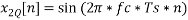
Figure 17 IQ Downconverter (Tsimenidis, 2016)
Upon these definitions, the components that we obtain could be represented in two separated graphs, each one of them representing a different component table.
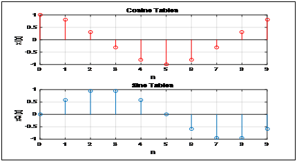
Figure 18 Sine and cosine table graphs
As for the index control of look-up table, we decide to use for loop to generate x2I[n] and x2Q[n], storing and transporting data to corresponding files as x2I.h and x2Q.h. These files will be used later to perform the conversion of values.
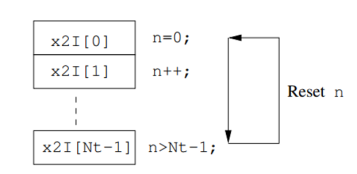
Figure 19 Index control flow (Tsimenidis, 2016)
After understanding the principle, we defined all of variables and initialized them to zero inside the main, and select the appropriate value of some variables such as state_mf, coeffs_mf and N_mf.Same as the picture over, the original data from bandpass output is also separated into two filters: Matched Filter I and Matched Filter Q, and the coefficients of the filters are the same with the original one. The benefit of using the lookup-table oscillators (setting x2 into x2I and x2Q) is to decrease the time of simulation because of the lower required sampling rate. We can use via lookup table method to call them from x2I.h and x2Q.h, so that we can use it more efficiently in Matlab instead of shifting itself. And then, we multiplied x1 to x2I[n] and x2Q[n] one by one by using another for loop and got x3I and x3Q.Besides,the code of matched filter had been given by tutors and got x4I and x4Q.
{x4I=fir(x3I,coeff_mf,state_mf_I,N_mf);Â //match filter I }
{x4Q=fir(x3I,coeff_mf,state_mf_Q,N_mf);Â //match filter I }
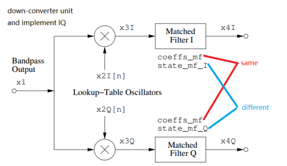
Figure 20 Filter comparison (Tsimenidis, 2016)
We monitored and recorded x3I and x3Q in PicoScope and print screen. The wave of them spinning fixed at the origin point so three of these blows were selected to describe this wave batter.
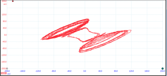
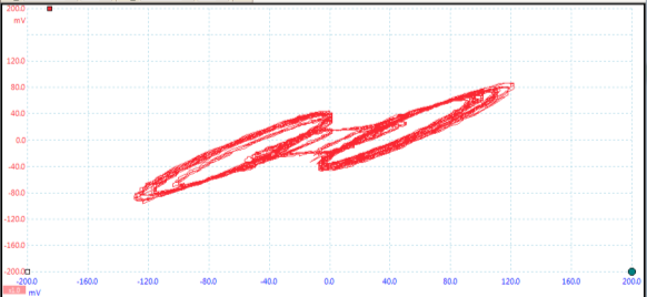
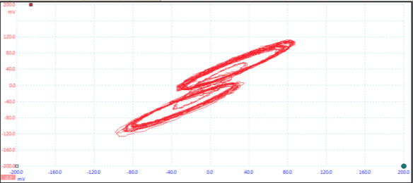
Figure 21 Down-conversion: x3I vs. x3Q counter clockwise
After this, we can visualize the outputs of each one of the filters, now we are going to plot in the figure x4I and x4Q, obtaining:
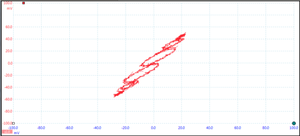
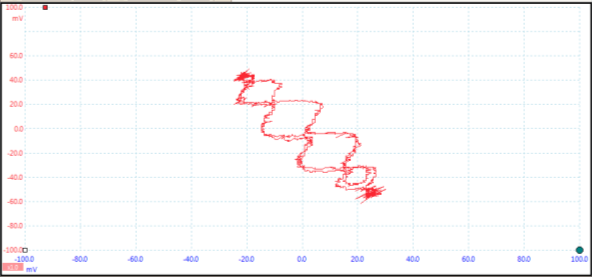
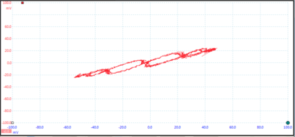
Figure 22 Down-conversion: x4I vs. x4Q counter clockwise
3.2. Symbol synchronization
After IQ down-converter, the next stage is symbol synchronization. To achieve this, we create x5I[n] and x5Q[n] and sent x4I, x4Q one sample at the time. The procedure that we should do in this section is similar to the one seen in the non-coherent detection, however we must consider two buffers instead of one, one for I and other for Q parts.
The sum of the above established energies will correspond to the energy that can be seen as the total energy of the signal, which is similar to lab of the symbol synchronization for the non-coherent receiver.
The corresponding calculations to obtain the signals after the symbol synchronization process are defined as:

Then, plotting the results obtained, we see the following figure:
Due to synchronization problems, we threated the jitter that was causing these inconsistences using the averaging approach, as described in the follows:
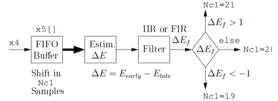
Figure 24 Averaging approach to overcome the jitter (Tsimenidis, 2016)
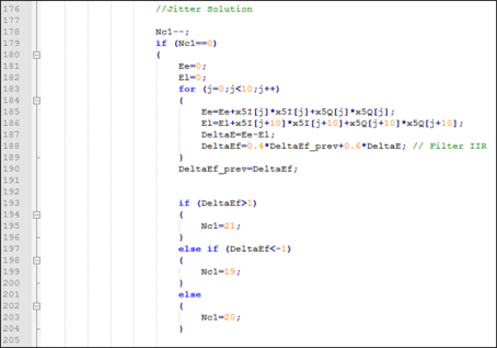
Figure 25 Code to solve the jitter
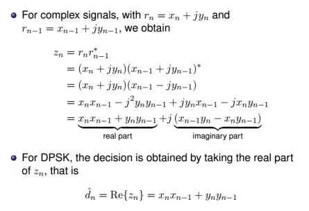
3.3. Differential coherent demodulator
In this section, we will implement a differential detector, also called a differential coherent demodulator.
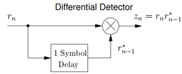
Figure 26 Principle of the differential detector (Tsimenidis, 2016)
At first, we declare and initialize appropriately the required variables and define  .In this differential detector,
 need to multiply
  ,1 symbol delay by .
|
N |
|
|
|
|
N=1 |
|
|
|
|
N=2 |
|
|
|
|
N=3 |
|
|
|


After this, we defined x6I_prev and x6Q_prev to deal with this problem and let x6I_prev and x6Q_prev denote the values of x6I and x6Q from the previous symbol. It is very important to initialize them to zero at the declaration because we know  . (Tsimenidis, 2016)

x6I_prev=x6I;
x6Q_prev=x6Q
On the same time,


dI contains the first two terms which stand for the In-phase part and dQ which contains the last two terms which stand for the Quadrature part.
Hard decision is then achieved by deciding whether the dI value is positive or negative, with a negative value indicating that a logic 1 was transmitted which might be used in the next step that is frame synchronization and message detection.
Now we obtain the plot showi
Cite This Work
To export a reference to this article please select a referencing stye below:
Related Services
View all


DMCA / Removal Request
If you are the original writer of this essay and no longer wish to have your work published on UKEssays.com then please click the following link to email our support team:
Request essay removal