Quantitative Reasoning and Analysis: An Overview
| ✅ Paper Type: Free Essay | ✅ Subject: Statistics |
| ✅ Wordcount: 383 words | ✅ Published: 23 Apr 2018 |
- Frances Roulet
State the statistical assumptions for this test.
Frankfort-Nachmias & Nachmias (2008) refers to the statistical inference as the procedure about population characteristics based on a sample result. In the understanding of some of these characteristics of the population, a random sample is taken, and the properties of the same is study, therefore, concluding by indicating if the sample are representative of the population.
An estimator function must be chosen for the characteristic of the population to be a study. Once the estimator function is applied to the sample, the results will an estimate. When using the appropriate statistical test, it can determine whether this estimate is based only on chance and if so, this will be called the null hypothesis and symbolized as H0 (Frankfort-Nachmias & Nachmias, 2008). This is the hypothesis that is tested directly, and if rejected as being unlikely, the research hypothesis is supported. The complement of the null hypothesis is known as the alternative hypothesis. This alternative hypothesis is symbolized as Ha. The two hypothesis are complementary; therefore, it is sufficient to define the null hypothesis.
According to Frankfort-Nachmias & Nachmias (2008) the need for two additional hypotheses arises out of a logical necessity. The null hypothesis responded to the negative inference in order to avoid the fallacy of affirming the consequent; in other words the researcher is required to eliminate the false hypotheses instead of accepting true ones.
Once the null hypothesis has been formulated, the researcher continues to test it against the sample result. The investigator, test the null hypothesis by comparing the sample result to a statistical model that provides the probability of observing such a result. This statistical model is called as the sampling distribution (Frankfort-Nachmias & Nachmias, 2008). Sampling distribution allows the researcher to estimate the probability of obtaining the sample result. This probability is well known as the level of significance or symbolically designated as α (alpha); which, is also the probability of rejecting a true hypothesis, H0 is rejected even though it is true (false positive) becomes Type I error. Normally, a significance level of α = .05 is used (even though at times other levels such as α = .01 may be used). This means that we are willing to tolerate up to 5% of type I errors. The probability value (value p) of the statistic used to test the null hypothesis, considering that, p <α then the null hypothesis will be rejected; meanwhile, the acceptance level of Type II error, H0 is not rejected even though it is false (false negative) is designated as β (beta) (Frankfort-Nachmias & Nachmias, 2008). In fact, the critical region is a part of the sample that is consistent with the rejection of the null hypothesis. The significance level is the probability that the test statistic will decline within the critical region when the null hypothesis is assumed. The critical region is represented as a region under a curve for continuous distributions (Frankfort-Nachmias & Nachmias, 2008).

The most common approach for testing a null hypothesis is to select a statistic based on a sample of fixed size, calculate the value of the statistic for the sample and then reject the null hypothesis if and only the statistic falls in the critical region. The statistical test may be one-tailed or two-tailed. In a one-tailed hypothesis testing specifies a direction of the statistical test, extreme results lead to the rejection of the null hypothesis and can be located at either tail (Zaiontz, 2015). An example of this is observed in the following graphic:
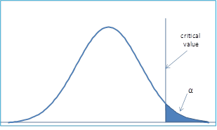 Figure 1 – Critical region is the right tail
The critical value here is the right (or upper) tail. It is quite possible to have one-sided tests where the critical value is the left (or lower) tail.
In a two-tailed test, the region of rejection is located in both the left and right tails. Indeed, the two-tailed hypothesis testing doesn’t specify a direction of the test.
An example of this is illustrated graphically as follows:
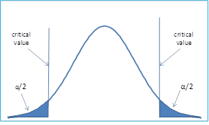 Figure 2 – Critical region is the left tail.
This possibility is being taken care as a two-tailed test using with the critical region and consisting of both the upper and lower tails. The null hypothesis is rejected if the test statistic falls in either side of the critical region. And, to achieve a significance level of α, the critical region in each tail must have a size α/2.
The statistical power is 1-β, the power is the probability of rejecting a false null hypothesis. While the significance level for Type I error of α =.05 is typically used, generally the target for β is .20 or .10 and .80 or .90 is used as the target value for power (Zaiontz, 2015).
When reading of the effect size, it is important to comprehend that an effect is the size of the variance explained by statistical model. This situation is opposed to the error, which is the size of the variance not explained by the model. The effect size is a standardized measure of the magnitude of an effect. As it is standardized, by comparing the effects across different studies with different variables and different scales can be done. For example, the differences in the mean between two groups can be expressed in term of the standard deviation. The effect size of 0.5 signifies that the difference between the means is half of the standard deviation. The most common measures of effect size are Cohen’s d, Pearson’s correlation coefficient r, and the odds ratio, even though there are other measures also to be used.
Cohen’s d is a statistic which is independent of the sample size and is defined as  , where m1 and m2 represent two means and σpooled is some combined value for the standard deviation (Zaiontz, 2015).
The effect size given by d is normally viewed as small, medium or large as follows:
• d = 0.20 – small effect
• d = 0.50 – medium effect
• d = 0.80 – large effect
The following value for d in a single sample hypothesis testing of the mean:
 .
.
The main goal is to provide a solid sense of whether a difference between two groups is meaningfully large, independent of whether the difference is statistically significant.
On the other hand, t Test effect size indicates whether or not the difference between two groups’ averages is large enough to have practical meaning, whether or not it is statistically significant.
However, a t test questions whether a difference between two groups’ averages is unlikely to have occurred because of random chance in sample selection. It is expected that the difference is more likely to be meaningful and “real” if:
- the difference between the averages is large,
- the sample size is large, and,
- responses are consistently close to the average values and not widely spread out (the standard deviation is low).
A statistically significant t test result becomes one in which a difference between two groups is unlikely to have occurred because the sample happened to be atypical. Statistical significance is determined by the size of the difference between the group averages, the sample size, and the standard deviations of the groups. It is suggested, for practical purposes, that statistical significance suggests that the two larger populations from which the sample are “actually” different (Zaiontz, 2015).
The t test’s statistical significance and the t test’s effect size are the two primary outputs of the t test. The t statistic analysis is used to test hypotheses about an unknown population mean (µ) when the value of the population variance (σ2) is unknown. The t statistic uses the sample variance (S2) as an estimate of the population variance (σ2) (Zaiontz, 2015).
In the t test there are two assumptions that must be met, in order to have a justification for this statistical test:
- Sample observations must be independent. In other words, there is no relationship between or among any of the observations (scores) in the sample.
- The population from which a sample has been obtained must be normally distributed.
- Must have continuous dependent variable.
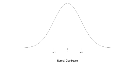
- Dependent variable has a normal distribution, with the same variance, σ2, in each group (as though the distribution for group A were merely shifted over to become the distribution for group B, without changing shape):
 Bottom of Form
Top of Form
Bottom of Form
Bottom of Form
Note: σ, “sigma”, the scale parameter of the normal distribution, also known as the population standard deviation, is easy to see on a picture of a normal curve. Located one σ to the left or right of the normal mean are the two places where the curve changes from convex to concave (the second derivative is zero) (Zaiontz, 2015).
The data set selected was from lesson 24.
The independent variable: Talk.
The dependent variable: Stress.
Hypotheses.
Null hypothesis: H0:  1- 2 = 0;
There is no difference between talk and level of stress.
In the null hypothesis, the Levene’s Test for equality of variances is H0: p= 0.5.
Alternative hypothesis: Ha: 1- 2 = 0;
There is difference between level of stress and talk.
In the alternative hypothesis, the Levene’s Test for equality of variances is Ha: p<> 0.5.
Statistical Report
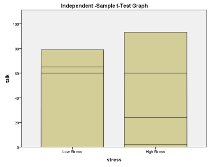
The group statistics of the independent samples test indicated that low stress (n=15, m=45.20, SD=24.969, SE=6.447) scored higher than the high stress (n=15, m=22.07, SD=27.136, SE=7.006).
|
Group Statistics |
|||||
|
stress |
N |
Mean |
Std. Deviation |
Std. Error Mean |
|
|
talk |
Low Stress |
15 |
45.20 |
24.969 |
6.447 |
|
High Stress |
15 |
22.07 |
27.136 |
7.006 |
The sample size of this results is of N=30, and its TS=t30=2.430; pvalue=.881 <.05 provided evidence to retain the null hypothesis. Therefore it is not statistically significant, if p.05 < indicating that the variances or standard deviations are the same in all probability.
|
Independent Samples Test |
||||||||||
|
Levene’s Test for Equality of Variances |
t-test for Equality of Means |
|||||||||
|
F |
Sig. |
t |
df |
Sig. (2-tailed) |
Mean Difference |
Std. Error Difference |
95% Confidence Interval of the Difference |
|||
|
Lower |
Upper |
|||||||||
|
Talk |
Equal variances assumed |
.023 |
.881 |
2.430 |
28 |
.022 |
23.133 |
9.521 |
3.630 |
42.637 |
|
Equal variances not assumed |
2.430 |
27.808 |
.022 |
23.133 |
9.521 |
3.624 |
42.643 |
Levene’s Test for equality of variances reports that the P<.05 >P.05, the analysis for this test p=.881 is significance, therefore, is assumed that the variances are equal. There is no evidence that the variances of the two groups are different from each other. In comparing the P-value of .881 to .05 we find that there is no evidence to reject the null hypothesis, therefore, the H0 is not rejected.
Graph.
SPSS syntax and output files.
T-Test
T-TEST GROUPS=stress(1 2)
/MISSING=ANALYSIS
/VARIABLES=talk
/CRITERIA=CI(.95).
|
Notes |
||
|
Output Created |
28-JAN-2015 00:27:21 |
|
|
Comments |
||
|
Input |
Data |
C:UsersFrances RoulAppDataLocalTempTemp1_new_datasets_7e-10.zip ew_datasets_7e ew_datasets_7eLesson 24 Data File 1.sav |
|
Active Dataset |
DataSet3 |
|
|
Filter |
|
|
|
Weight |
|
|
|
Split File |
|
|
|
N of Rows in Working Data File |
30 |
|
|
Missing Value Handling |
Definition of Missing |
User defined missing values are treated as missing. |
|
Cases Used |
Statistics for each analysis are based on the cases with no missing or out-of-range data for any variable in the analysis. |
|
|
Syntax |
T-TEST GROUPS=stress(1 2) /MISSING=ANALYSIS /VARIABLES=talk /CRITERIA=CI(.95). |
|
|
Resources |
Processor Time |
00:00:00.02 |
|
Elapsed Time |
00:00:00.01 |
[DataSet3] C:UsersFrances RoulAppDataLocalTempTemp1_new_datasets_7e-10.zipnew_datasets_7enew_datasets_7eLesson 24 Data File 1.sav
GGraph
* Chart Builder.
GGRAPH
/GRAPHDATASET NAME=”graphdataset” VARIABLES=stress talk MISSING=LISTWISE REPORTMISSING=NO
/GRAPHSPEC SOURCE=INLINE.
BEGIN GPL
SOURCE: s=userSource(id(“graphdataset”))
DATA: stress=col(source(s), name(“stress”), unit.category())
DATA: talk=col(source(s), name(“talk”))
GUIDE: axis(dim(1), label(“stress”))
GUIDE: axis(dim(2), label(“talk”))
GUIDE: text.title(label(“Independent -Sample t-Test Graph”))
SCALE: cat(dim(1), include(“1”, “2”))
SCALE: linear(dim(2), include(0))
ELEMENT: interval(position(stress*talk), shape.interior(shape.square))
END GPL.
|
Notes |
||
|
Output Created |
28-JAN-2015 01:31:16 |
|
|
Comments |
||
|
Input |
Data |
C:UsersFrances RoulAppDataLocalTempTemp1_new_datasets_7e-10.zip ew_datasets_7e ew_datasets_7eLesson 24 Data File 1.sav |
|
Active Dataset |
DataSet3 |
|
|
Filter |
|
|
|
Weight |
|
|
|
Split File |
|
|
|
N of Rows in Working Data File |
30 |
|
|
Syntax |
GGRAPH /GRAPHDATASET NAME=”graphdataset” VARIABLES=stress talk MISSING=LISTWISE REPORTMISSING=NO /GRAPHSPEC SOURCE=INLINE. BEGIN GPL SOURCE: s=userSource(id(“graphdataset”)) DATA: stress=col(source(s), name(“stress”), unit.category()) DATA: talk=col(source(s), name(“talk”)) GUIDE: axis(dim(1), label(“stress”)) GUIDE: axis(dim(2), label(“talk”)) GUIDE: text.title(label(“Independent -Sample t-Test Graph”)) SCALE: cat(dim(1), include(“1”, “2”)) SCALE: linear(dim(2), include(0)) ELEMENT: interval(position(stress*talk), shape.interior(shape.square)) END GPL. |
|
|
Resources |
Processor Time |
00:00:00.14 |
|
Elapsed Time |
00:00:00.14 |
[DataSet3] C:UsersFrances RoulAppDataLocalTempTemp1_new_datasets_7e-10.zipnew_datasets_7enew_datasets_7eLesson 24 Data File 1.sav
References
Frankfort-Nachmias, C., & Nachmias, D. (2008). Research methods in the social sciences. (Seventh Edition). New York, N.Y.: Worth Publishers.
Zaiontz, C. (2015). Real statistics using Excel. www.real-statistics.com
Laureate Education, Inc. (Executive Producer). (2009n). The t test for related samples. Baltimore: Author.
Cite This Work
To export a reference to this article please select a referencing stye below:
Related Services
View all


DMCA / Removal Request
If you are the original writer of this essay and no longer wish to have your work published on UKEssays.com then please click the following link to email our support team:
Request essay removal